
Recursion has something to do with infinity. I know recursion has something to do with infinity. I think I know recursion has something to do with infinity. He is sure I think I know recursion has something to do with infinity. We doubt he is sure I think I know ... We think that you think that we convinced you now that we can go on forever with this example of a recursion from natural language. Recursion is not only a fundamental feature of natural language, but of the human cognitive capacity. Our way of thinking is based on a recursive thinking processes. Even with a very simple grammar, like "An English sentence contains a subject and a predicate, and a predicate contains a verb, an object and a complement", we can demonstrate the infinite possibilities of the natural language. The cognitive scientist and linguist Stephen Pinker phrases it like this: "With a few thousand nouns that can fill the subject slot and a few thousand verbs that can fill the predicate slot, one already has several million ways to open a sentence. The possible combinations quickly multiply out to unimaginably large numbers. Indeed, the repertoire of sentences is theoretically infinite, because the rules of language use a trick called recursion. A recursive rule allows a phrase to contain an example of itself, as in She thinks that he thinks that they think that he knows and so on, ad infinitum. And if the number of sentences is infinite, the number of possible thoughts and intentions is infinite too, because virtually every sentence expresses a different thought or intention."1
We have to stop our short excursion to the use of recursion in natural language to come back to recursion in computer science and programs and finally to recursion in the programming language Python.
The adjective "recursive" originates from the Latin verb "recurrere", which means "to run back". And this is what a recursive definition or a recursive function does: It is "running back" or returning to itself. Most people who have done some mathematics, computer science or read a book about programming will have encountered the factorial, which is defined in mathematical terms as
n! = n * (n-1)!, if n > 1 and 0! = 1
It's used so often as an example for recursion because of its simplicity and clarity. We will come back to it in the following.
Definition of Recursion
Recursion is a method of programming or coding a problem, in which a function calls itself one or more times in its body. Usually, it is returning the return value of this function call. If a function definition satisfies the condition of recursion, we call this function a recursive function.
Termination condition:
A recursive function has to fulfil an important condition to be used in a program: it has to terminate. A recursive function terminates, if with every recursive call the solution of the problem is downsized and moves towards a base case. A base case is a case, where the problem can be solved without further recursion. A recursion can end up in an infinite loop, if the base case is not met in the calls.
Example:
4! = 4 * 3!

3! = 3 * 2!

2! = 2 * 1
Replacing the calculated values gives us the following expression
4! = 4 * 3 * 2 * 1
Generally we can say: Recursion in computer science is a method where the solution to a problem is based on solving smaller instances of the same problem.
Recursive Functions in Python
Now we come to implement the factorial in Python. It's as easy and elegant as the mathematical definition.
def factorial(n):if n == 1:else:return 1return n * factorial(n-1)
We can track how the function works by adding two print() functions to the previous function definition:
def factorial(n):print("factorial has been called with n = " + str(n))if n == 1: return 1 else:print("intermediate result for ", n, " * factorial(" ,n-1, "): ",res)res = n * factorial(n-1) return resprint(factorial(5))
This Python script outputs the following results:
factorial has been called with n = 5factorial has been called with n = 4factorial has been called with n = 2factorial has been called with n = 3 factorial has been called with n = 1intermediate result for 3 * factorial( 2 ): 6intermediate result for 2 * factorial( 1 ): 2 intermediate result for 4 * factorial( 3 ): 24120intermediate result for 5 * factorial( 4 ): 120
Let's have a look at an iterative version of the factorial function.
def iterative_factorial(n):result = 1result *= ifor i in range(2,n+1):return result
It is common practice to extend the factorial function for 0 as an argument. It makes sense to define 0! to be 1, because there is exactly one permutation of zero objects, i.e. if nothing is to permute, "everything" is left in place. Another reason is that the number of ways to choose n elements among a set of n is calculated as n! divided by the product of n! and 0!.
All we have to do to implement this is to change the condition of the if statement:
def factorial(n):if n == 0:else:return 1return n * factorial(n-1)
The Pitfalls of Recursion
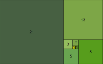
This subchapter of our tutorial on recursion deals with the Fibonacci numbers. What do have sunflowers, the Golden ratio, fir tree cones, The Da Vinci Code, the song "Lateralus" by Tool, and the graphic on the right side in common. Right, the Fibonacci numbers.
The Fibonacci numbers are the numbers of the following sequence of integer values:
0,1,1,2,3,5,8,13,21,34,55,89, ...
The Fibonacci numbers are defined by:
Fn = Fn-1 + Fn-2
with
F0 = 0 and F1 = 1
The Fibonacci sequence is named after the mathematician Leonardo of Pisa, who is better known as Fibonacci. In his book "Liber Abaci" (publishes 1202) he introduced the sequence as an exercise dealing with bunnies. His sequence of the Fibonacci numbers begins with F1 = 1, while in modern mathematics the sequence starts with F0 = 0. But this has no effect on the other members of the sequence.
The Fibonacci numbers are the result of an artificial rabbit population, satisfying the following conditions:
- a newly born pair of rabbits, one male, one female, build the initial population
- these rabbits are able to mate at the age of one month so that at the end of its second month a female can bring forth another pair of rabbits
- these rabbits are immortal
- a mating pair always produces one new pair (one male, one female) every month from the second month onwards
The Fibonacci numbers are the numbers of rabbit pairs after n months, i.e. after 10 months we will have F10 rabits.
The Fibonacci numbers are easy to write as a Python function. It's more or less a one to one mapping from the mathematical definition:
def fib(n):if n == 0:return 0elif n == 1:else:return 1return fib(n-1) + fib(n-2)
An iterative solution is also easy to write, though the recursive solution looks more like the definition:
def fibi(n):old, new = 0, 1if n == 0:for i in range(n-1):return 0old, new = new, old + newreturn new
If you check the functions fib() and fibi(), you will find out that the iterative version fibi() is a lot faster than the recursive version fib(). To get an idea of how much this "a lot faster" can be, we have written a script, which uses the timeit module, to measure the calls. To do this, we save the function definitions for fib and fibi in a file fibonacci.py, which we can import in the program (fibonacci_runit.py) below:
from timeit import Timert1 = Timer("fib(10)","from fibonacci import fib")for i in range(1,41): s = "fib(" + str(i) + ")"time1 = t1.timeit(3)t1 = Timer(s,"from fibonacci import fib") s = "fibi(" + str(i) + ")"print("n=%2d, fib: %8.6f, fibi: %7.6f, percent: %10.2f" % (i, time1, time2, time1/time2))t2 = Timer(s,"from fibonacci import fibi")time2 = t2.timeit(3)
time1 is the time in seconds it takes for 3 calls to fib(n) and time2 respectively the time for fibi(). If we look at the results, we can see that calling fib(20) three times needs about 14 milliseconds. fibi(20) needs just 0.011 milliseconds for 3 calls. So fibi(20) is about 1300 times faster then fib(20).
fib(40) needs already 215 seconds for three calls, while fibi(40) can do it in 0.016 milliseconds. fibi(40) is more than 13 millions times faster than fib(40).
n= 1, fib: 0.000004, fibi: 0.000005, percent: 0.81n= 2, fib: 0.000005, fibi: 0.000005, percent: 1.00n= 4, fib: 0.000008, fibi: 0.000005, percent: 1.62n= 3, fib: 0.000006, fibi: 0.000006, percent: 1.00 n= 5, fib: 0.000013, fibi: 0.000006, percent: 2.20n= 8, fib: 0.000047, fibi: 0.000008, percent: 5.79n= 6, fib: 0.000020, fibi: 0.000006, percent: 3.36 n= 7, fib: 0.000030, fibi: 0.000006, percent: 5.04 n= 9, fib: 0.000075, fibi: 0.000007, percent: 10.50n=13, fib: 0.000480, fibi: 0.000007, percent: 69.45n=10, fib: 0.000118, fibi: 0.000007, percent: 16.50 n=11, fib: 0.000198, fibi: 0.000007, percent: 27.70 n=12, fib: 0.000287, fibi: 0.000007, percent: 41.52 n=14, fib: 0.000780, fibi: 0.000007, percent: 112.83n=19, fib: 0.009219, fibi: 0.000011, percent: 840.59n=15, fib: 0.001279, fibi: 0.000008, percent: 162.55 n=16, fib: 0.002059, fibi: 0.000009, percent: 233.41 n=17, fib: 0.003439, fibi: 0.000011, percent: 313.59 n=18, fib: 0.005794, fibi: 0.000012, percent: 486.04 n=20, fib: 0.014366, fibi: 0.000011, percent: 1309.89n=26, fib: 0.253764, fibi: 0.000013, percent: 19352.05n=21, fib: 0.023137, fibi: 0.000013, percent: 1764.42 n=22, fib: 0.036963, fibi: 0.000013, percent: 2818.80 n=23, fib: 0.060626, fibi: 0.000012, percent: 4985.96 n=24, fib: 0.097643, fibi: 0.000013, percent: 7584.17 n=25, fib: 0.157224, fibi: 0.000013, percent: 11989.91 n=27, fib: 0.411353, fibi: 0.000012, percent: 34506.80n=34, fib: 11.980462, fibi: 0.000014, percent: 851689.83n=28, fib: 0.673918, fibi: 0.000014, percent: 47908.76 n=29, fib: 1.086484, fibi: 0.000015, percent: 72334.03 n=30, fib: 1.742688, fibi: 0.000014, percent: 123887.51 n=31, fib: 2.861763, fibi: 0.000014, percent: 203442.44 n=32, fib: 4.648224, fibi: 0.000015, percent: 309461.33 n=33, fib: 7.339578, fibi: 0.000014, percent: 521769.86n=40, fib: 215.091484, fibi: 0.000016, percent: 13465060.78n=35, fib: 19.426206, fibi: 0.000016, percent: 1216110.64 n=36, fib: 30.840097, fibi: 0.000015, percent: 2053218.13 n=37, fib: 50.519086, fibi: 0.000016, percent: 3116064.78 n=38, fib: 81.822418, fibi: 0.000015, percent: 5447430.08n=39, fib: 132.030006, fibi: 0.000018, percent: 7383653.09
What's wrong with our recursive implementation?
Let's have a look at the calculation tree, i.e. the order in which the functions are called. fib() is substituted by f().
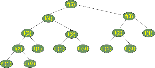
We can see that the subtree f(2) appears 3 times and the subtree for the calculation of f(3) two times. If you imagine extending this tree for f(6), you will understand that f(4) will be called two times, f(3) three times and so on. This means, our recursion doesn't remember previously calculated values.
We can implement a "memory" for our recursive version by using a dictionary to save the previously calculated values.
memo = {0:0, 1:1}def fibm(n):if not n in memo:memo[n] = fibm(n-1) + fibm(n-2)return memo[n]
We time it again to compare it with fibi():
from timeit import Timerfrom fibonacci import fibt1 = Timer("fib(10)","from fibonacci import fib")for i in range(1,41): s = "fibm(" + str(i) + ")"time1 = t1.timeit(3)t1 = Timer(s,"from fibonacci import fibm") s = "fibi(" + str(i) + ")"print("n=%2d, fib: %8.6f, fibi: %7.6f, percent: %10.2f" % (i, time1, time2, time1/time2))t2 = Timer(s,"from fibonacci import fibi")time2 = t2.timeit(3)
We can see that it is even faster than the iterative version. Of course, the larger the arguments the greater the benefit of our memoization:
n= 1, fib: 0.000011, fibi: 0.000015, percent: 0.73n= 2, fib: 0.000011, fibi: 0.000013, percent: 0.85n= 4, fib: 0.000012, fibi: 0.000015, percent: 0.79n= 3, fib: 0.000012, fibi: 0.000014, percent: 0.86 n= 5, fib: 0.000012, fibi: 0.000016, percent: 0.75n= 8, fib: 0.000011, fibi: 0.000018, percent: 0.61n= 6, fib: 0.000011, fibi: 0.000017, percent: 0.65 n= 7, fib: 0.000012, fibi: 0.000017, percent: 0.72 n= 9, fib: 0.000011, fibi: 0.000018, percent: 0.61n=13, fib: 0.000004, fibi: 0.000007, percent: 0.57n=10, fib: 0.000010, fibi: 0.000020, percent: 0.50 n=11, fib: 0.000011, fibi: 0.000020, percent: 0.55 n=12, fib: 0.000004, fibi: 0.000007, percent: 0.59 n=14, fib: 0.000004, fibi: 0.000008, percent: 0.52n=19, fib: 0.000004, fibi: 0.000009, percent: 0.45n=15, fib: 0.000004, fibi: 0.000008, percent: 0.50 n=16, fib: 0.000003, fibi: 0.000008, percent: 0.39 n=17, fib: 0.000004, fibi: 0.000009, percent: 0.45 n=18, fib: 0.000004, fibi: 0.000009, percent: 0.45 n=20, fib: 0.000003, fibi: 0.000010, percent: 0.29n=26, fib: 0.000004, fibi: 0.000011, percent: 0.34n=21, fib: 0.000004, fibi: 0.000009, percent: 0.45 n=22, fib: 0.000004, fibi: 0.000010, percent: 0.40 n=23, fib: 0.000004, fibi: 0.000010, percent: 0.40 n=24, fib: 0.000004, fibi: 0.000011, percent: 0.35 n=25, fib: 0.000004, fibi: 0.000012, percent: 0.33 n=27, fib: 0.000004, fibi: 0.000011, percent: 0.35n=34, fib: 0.000004, fibi: 0.000012, percent: 0.34n=28, fib: 0.000004, fibi: 0.000012, percent: 0.32 n=29, fib: 0.000004, fibi: 0.000012, percent: 0.33 n=30, fib: 0.000004, fibi: 0.000013, percent: 0.31 n=31, fib: 0.000004, fibi: 0.000012, percent: 0.34 n=32, fib: 0.000004, fibi: 0.000012, percent: 0.33 n=33, fib: 0.000004, fibi: 0.000013, percent: 0.30 n=35, fib: 0.000004, fibi: 0.000013, percent: 0.31n=40, fib: 0.000004, fibi: 0.000014, percent: 0.29n=36, fib: 0.000004, fibi: 0.000013, percent: 0.31 n=37, fib: 0.000004, fibi: 0.000014, percent: 0.29 n=38, fib: 0.000004, fibi: 0.000014, percent: 0.29n=39, fib: 0.000004, fibi: 0.000013, percent: 0.31
We can also define a recursive algorithm for our Fibonacci function by using a class with callabe instances, i.e. by using the special method __call__. This way, we will be able to hide the dictionary in an elegant way. We used a general approach which allows as to define also functions similar to Fibonacci, like the Lucas function:
class Fibonacci:def __init__(self, i1=0, i2=1):self.memo = {0:i1, 1:i2}if n not in self.memo:def __call__(self, n):self.memo[n] = self.__call__(n-1) + self.__call__(n-2)return self.memo[n] fib = Fibonacci() lucas = Fibonacci(2, 1)print(i, fib(i), lucas(i))for i in range(1, 16):
The program returns the following output:
1 1 12 1 34 3 73 2 46 8 185 5 118 21 477 13 2910 55 1239 34 7612 144 32211 89 19914 377 84313 233 52115 610 1364
The Lucas numbers or Lucas series are an integer sequence named after the mathematician François Édouard Anatole Lucas (1842–91), who studied both that sequence and the closely related Fibonacci numbers. The Lucas numbers have the same creation rule than the Fibonacci number, i.e. the sum of the two previous numbers, but the values for 0 and 1 are different.
More about Recursion in Python

If you want to learn more on recursion, we suggest that you try to solve the following exercises. Please do not peer at the solutions, before you haven't given your best. If you have thought about a task for a while and you are still not capable of solving the exercise, you may consult our sample solutions.
In our section "Advanced Topics" of our tutorial we have a comprehensive treatment of the game or puzzle "Towers of Hanoi". Of course, we solve it with a function using a recursive function. The "Hanoi problem" is special, because a recursive solution almost forces itself on the programmer, while the iterative solution of the game is hard to find and to grasp.
Exercises
- Think of a recusive version of the function f(n) = 3 * n, i.e. the multiples of 3
- Write a recursive Python function that returns the sum of the first
nintegers.(Hint: The function will be similiar to the factorial function!) - Write a function which implements the Pascal's triangle:11 11 2 11 3 3 11 4 6 4 11 5 10 10 5 1
- The Fibonacci numbers are hidden inside of Pascal's triangle. If you sum up the coloured numbers of the following triangle, you will get the 7th Fibonacci number:11 11 2 11 3 3 11 4 6 4 11 5 10 10 5 11 6 15 20 15 6 1Write a recursive program to calculate the Fibonacci numbers, using Pascal's triangle.
- Implement a recursive function in Python for the sieve of Eratosthenes.The sieve of Eratosthenes is a simple algorithm for finding all prime numbers up to a specified integer. It was created by the ancient Greek mathematician Eratosthenes.The algorithm to find all the prime numbers less than or equal to a given integer n:
- Create a list of integers from two to n: 2, 3, 4, ..., n
- Start with a counter i set to 2, i.e. the first prime number
- Starting from i+i, count up by i and remove those numbers from the list, i.e. 2*i, 3*i, 4*i, aso..
- Find the first number of the list following i. This is the next prime number.
- Set i to the number found in the previous step
- Repeat steps 3 and 4 until i is greater than n. (As an improvement: It's enough to go to the square root of n)
- All the numbers, which are still in the list, are prime numbers
- Write a recursive function find_index(), which returns the index of a number in the Fibonacci sequence, if the number is an element of this sequence and returns -1 if the number is not contained in it, i.e.
fib(find_index(n)) == n
- The sum of the squares of two consecutive Fibonacci numbers is also a Fibonacci number, e.g. 2 and 3 are elements of the Fibonacci sequence and 2*2 + 3*3 = 13 corresponds to Fib(7).Use the previous function to find the position of the sum of the squares of two consecutive numbers in the Fibonacci sequence.Mathematical explanation:Let a and b be two successive Fibonacci numbers with a prior to b. The Fibonacci sequence starting with the number "a" looks like this:0 a1 b2 a + b3 a + 2b 4 2a + 3b6 5a + 8b5 3a + 5bWe can see that the Fibonacci numbers appear as factors for a and b. The n-th element in this sequence can be calculated with the following formula:
F(n) = Fib(n-1)* a + Fib(n) * b
From this we can conclude that for a natural number n, n>1, the following holds true:Fib(2*n + 1) = Fib(n)**2 + Fib(n+1)**2
You can easily see that we would be inefficient, if we strictly used this algorithm, e.g. we will try to remove the multiples of 4, although they have been already removed by the multiples of 2. So it's enough to produce the multiples of all the prime numbers up to the square root of n. We can recursively create these sets.
Solutions to our Exercises
- Solution to our first exercise on recursion:Mathematically, we can write it like this:f(1) = 3,f(n+1) = f(n) + 3A Python function can be written like this:def mult3(n):if n == 1:return 3else:return mult3(n-1) + 3Towers of Hanoi for i in range(1,10):print(mult3(i))
- Solution to our second exercise:def sum_n(n):if n== 0:return 0else:return n + sum_n(n-1)
- Solution for creating the Pacal triangle:def pascal(n):if n == 1:return [1]else: line = [1]previous_line = pascal(n-1)for i in range(len(previous_line)-1):line += [1]line.append(previous_line[i] + previous_line[i+1]) return lineprint(pascal(6))Alternatively, we can write a function using list comprehension:def pascal(n):if n == 1:return [1]else:line = [ p_line[i]+p_line[i+1] for i in range(len(p_line)-1)]p_line = pascal(n-1)line.append(1)line.insert(0,1) return lineprint(pascal(6))
- Producing the Fibonacci numbers out of Pascal's triangle:def fib_pascal(n,fib_pos):if n == 1:fib_sum = 1 if fib_pos == 0 else 0line = [1] else:(previous_line, fib_sum) = fib_pascal(n-1, fib_pos+1)line = [1]line.append(previous_line[i] + previous_line[i+1])for i in range(len(previous_line)-1):fib_sum += line[fib_pos]line += [1] if fib_pos < len(line):return fib_pascal(n,0)[1]return (line, fib_sum) def fib(n):print(fib(i))# and now printing out the first ten Fibonacci numbers:for i in range(1,10):
- The following program implements the sieve of Eratosthenes according to the rules of the task in an iterative way. It will print out the first 100 prime numbers.from math import sqrtdef sieve(n):# returns all primes between 2 and nprimes = list(range(2,n+1)) max = sqrt(n) num = 2i += numwhile num < max: i = num while i <= n: if i in primes:breakprimes.remove(i) for j in primes: if j > num: num = j return primesprint(sieve(100))But this chapter of our tutorial is about recursion and recursive functions, and we have demanded a recursive function to calculate the prime numbers. To understand the following solution, you may confer our chapter about List Comprehension:from math import sqrtdef primes(n):return []if n == 0:return []elif n == 1: else:p = primes(int(sqrt(n)))no_p = [j for i in p for j in range(i*2, n + 1, i)]return pp = [x for x in range(2, n + 1) if x not in no_p]print(primes(100))
- memo = {0:0, 1:1}def fib(n):if not n in memo:memo[n] = fib(n-1) + fib(n-2)return memo[n]""" finds the natural number i with fib(i) = n """def find_index(*x): if len(x) == 1:# find index starting from 0# started by user return find_index(x[0],0) else:elif n == m:n = fib(x[1]) m = x[0] if n > m: return -1 return x[1]return find_index(m,x[1]+1)else:
- # code from the previous example with the functions fib() and find_index()print(" index of a | a | b | sum of squares | index ")for i in range(15):print("=====================================================") square = fib(i)**2 + fib(i+1)**2print( " %10d | %3d | %3d | %14d | %5d " % (i, fib(i), fib(i+1), square, find_index(square)))The result of the previous program looks like this:index of a | a | b | sum of squares | index=====================================================0 | 0 | 1 | 1 | 12 | 1 | 2 | 5 | 51 | 1 | 1 | 2 | 3 3 | 2 | 3 | 13 | 76 | 8 | 13 | 233 | 134 | 3 | 5 | 34 | 9 5 | 5 | 8 | 89 | 11 7 | 13 | 21 | 610 | 1511 | 89 | 144 | 28657 | 238 | 21 | 34 | 1597 | 17 9 | 34 | 55 | 4181 | 19 10 | 55 | 89 | 10946 | 21 12 | 144 | 233 | 75025 | 2513 | 233 | 377 | 196418 | 27 14 | 377 | 610 | 514229 | 29
1 Stephen Pinker, The Blank Slate, 2002

No comments:
Post a Comment